Running the calculation

The ORCA manual, and the ORCA input library, should be consulted for instructions on how to run a TD-DFT calculation, or any sort of CI calculation.

Understanding the result

ORCA will print the information you need to the output file in a section with the following header

         ABSORPTION SPECTRUM VIA TRANSITION ELECTRIC DIPOLE MOMENTS
-----------------------------------------------------------------------------
State   Energy    Wavelength  fosc         T2        TX        TY        TZ
        (cm-1)      (nm)                 (au**2)    (au)      (au)      (au)
-----------------------------------------------------------------------------

We only need the Energy and fosc entries to plot a spectrum. The fosc column contains the oscillator strength of each transition. In order to understand what this means, recall the integrated absorption coefficient of a given absorption band

Where $n$ is concentration $[\mathrm{mol \ m^{-3}}]$, $l$ is path length $[\mathrm{m}]$, $A_\mathrm{e}$ is the napierian absorbance, $\alpha_\mathrm{e}$ is the napierian absorption coefficient $[\mathrm{m^2 \ mol^{-1}}]$, $I$ and $I_0$ are the transmitted and incident radiation intensity respectively, and $\widetilde{\nu}$ is the wavenumber $[\mathrm{cm}^{-1}]$.

The oscillator strength $f$ is defined as the ratio of $\mathcal{A}_\mathrm{e}$ for a given band to the (constant) value for that of a harmonically oscillating electron.

and usually has a value between 0 and 1. In order to plot the spectrum, we need to convert $f$ back into $\mathcal{A}_\mathrm{e}^\mathrm{ORCA}$ since this tells us how large each absorption band will be.

An explanation of the oscillator strength can be found on Pages 80 and 81 of Barrow’s Introduction to Molecular Spectroscopy.

Plotting a spectrum

To generate the UV-Vis spectrum orca_mapspc uses an area-normalised Lorentzian lineshape $L(x)$ for each transition

where $\Gamma$ is the full-width-at-half-maximum (FWHM) of the curve, $x$ is the wavenumber of the incident radiation, and $x_0$ is the wavenumber of the transition.

For a given transition, the corresponing Lorentzian is multiplied by the linear integrated absorption coefficent $\mathcal{A}^\mathrm{ORCA}$ obtained by dividing $\mathcal{A}_\mathrm{e}^\mathrm{ORCA} \ [\mathrm{1000 \ cm \ mol^{-1}}]$ by $\ln(10)$. The multiplication of $L(x) \ [\mathrm{cm}]$ by $\mathcal{A}^\mathrm{ORCA} \ \ [\mathrm{1000 \ cm \ mol^{-1}}]$ gives a function with units of $[\mathrm{1000 \ cm^{2} \ mol^{-1}}] = [\mathrm{L \ mol^{-1} \ cm^{-1}}] = [\mathrm{M^{-1} \ cm^{-1}}]$, i.e. common units of the linear molar extinction coefficient $\epsilon$.

To combine all of the transitions as a single spectrum, simply sum $L(x) \cdot \mathcal{A}^\mathrm{ORCA}$ for each transition, and plot against wavenumber.

What about Velocity?

You might have noticed that ORCA prints an identical absorption spectrum table with the title

         ABSORPTION SPECTRUM VIA TRANSITION VELOCITY DIPOLE MOMENTS

which contains an identical set of transitions with slightly different oscillator strengths. This stems from the use of a different operator in calculating transition intensities which should give equivalent results, but rarely does due to the approximations used in quantum chemistry.

In order to calculate the oscillator strength of a transition between two states we need to know the value of the transition dipole moment for that transition.

The transition dipole moment is a matrix element of the dipole operator

In the case of the electric dipole moment and a particle in three-dimensions

where $q$ is the charge of the particle, and $\mathbf{r}$ the position operator.

The position operator and Hamiltonian operator have the well-known commutation relation

This can be obtained from the derivation for a single dimension

where

and

Alternatively $\left[\hat{H}, \mathbf{r}\right]$ can be evaluated directly

so then

Meaning that we can obtain transition dipole moment values by either computing the position operator directly, or by computing the velocity operator and using the above relationship.

Due to the number of approximations used in computational chemistry these two approaches rarely give the same answer. Therefore, ORCA and orca_mapspc allow the user to choose which value to use, and by default orca_mapspc uses the position form which they refer to as the electric dipole.

The Zeeman effect

$\newcommand{\tensor}[1]{\bar{\bar{#1}}}$

The magnetic moment $\vec{\mu}$ of a particle is a vector quantity and is proportional to the particle’s spin $\vec{S}$, with a dimensionless proportionality constant called the $g$ value. For an single isolated electron, the free electron $g$ value $g_\mathrm{e}$ is used.

where $\mu_\mathrm{B}$ is the Bohr magneton, which is a constant that essentially accounts for the units of the magnetic moment.

Magnetic moments can interact with magnetic fields $\vec{B}$ in a process known as the Zeeman effect, and this interaction is described by the Zeeman Hamiltonian

where the hat denotes the operator nature of the spin. If $\vec{B}$ and $\hat{\vec{S}}$ are known then the energies of the electronic spin states can be calculated. The vector operator $\hat{\vec{S}}$ is made up of spin operators for the three cartesian axes

where $\mathrm{T}$ indicates the transpose and the field vector $\vec{B}$ has components along $x$, $y$, and $z$

so the dot-product in $\hat{H}_\mathrm{Zee}$ can be evaluated to give

As an example, we can define $B_x=B_y=0\neq B_z$ so that $\hat{H}_\mathrm{Zee}$ becomes

and from this it is trivial to obtain the (hopefully) familiar equation for the energy of the electron when its spin is aligned either with or against the magnetic field (Zeeman splitting)

But what if the system is not a free electron? Very often electronic spins are confined to molecules and ions, and so the electrons experience a variety of potentials and fields. To account for this, the $g$ value can be modified and becomes a so called phenomenological quantity since it describes the interaction of spin states with a field, but doesnt really explain how or why. This phenomenological usage could even be taken a step further, since experimentally one might find that $g$ changes as a function of direction, and so $g$ is more generally represented by a tensor $\tensor{g}$ which has components $g_{\alpha,\beta}$ describing the effect of an arbitrarily oriented magnetic field on a set of spin states.

and so the Hamiltonian is

So in short: The g-tensor is a compact method for describing the effect of a magnetic field on a two level system (or more specifically a (pseudo) spin‑1/2 doublet) and contains a set of values $g_{\alpha, \beta}$.

One particularly useful feature of this (3x3) tensor is that it describes real space, and so if we find its “principal axes” (eigenvectors), we can then describe how readily this pair of states will be affected by a magnetic field in a given cartesian direction. Let’s pick a more interesting pair of states to look at, and then revisit this idea.

Crystal Fields

The electronic structures of lanthanide qubits and SMMs are often discussed in terms of the Hund’s rule ground term of the lanthanide in question. For example, Dy(III) is commonly used in SMMs and has a $^6 \mathrm{H}$ Hund’s rule ground term arising from its 4f⁹ electron configuration. Within this term the $J=15/2$ multiplet is lowest in energy, and contains a set of 16 $m_J$ states which are degenerate in the absence of any crystal or magnetic field. When such fields are applied, this degeneracy is lifted, and in the case of the crystal field (CF), this effect can be described using a CF Hamiltonian

where $\theta^k$ are a set of numerical factors which are constant for a given lanthanide ion, $B_k^q$ is a crystal field parameter which is unique to a given system, and $\hat{O}_k^q$ is a Stevens operator that can be calculated from the angular momentum operators $\hat{J}_i, \hat{J}^2 \ \ (i = x, y, z, +, -)$.

Considering a (hypothetical) perfectly axial CF allows $\hat{H}_\mathrm{CF}$ to be reduced to just the terms with $q=0$, and a further simplification can come from only including terms with $k=2,4,6$, since terms with $k>6$ make little difference to the states. Inputting the values $B_2^0 = 1000 \ \mathrm{cm}^{-1}$, $B_4^0 = 100 \ \mathrm{cm}^{-1}$, and $B_6^0 = 10 \ \mathrm{cm}^{-1}$ into the above Hamiltonian and diagonalising the resulting matrix representation yields a set of crystal field wavefunctions $\psi_i$ (Figure 1).

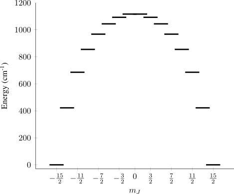
Figure 1: States of the J = 15/2 multiplet of Dy(III) in a perfectly axial crystal field.

In this example there are 8 pairs of degenerate states (doublets) with opposite values of $m_J$. The low energy (< 1000 cm^-1) doublets are well separated from each other, and so each doublet could be treated as a pseudo $S=1/2$ system with its own $\tensor{g}$. Then, the main magnetic axes of each doublet could be quantified and visualised, and we could start gain insight into how the molecular structure affects the electronic states.

Finding the pseudospin g values

The question is of course, how are the elements of $\tensor{g}$ found? We could apply a magnetic field $\vec{B}$ to our CF states and record how they change as the orientation of $\vec{B}$ is varied, but this is a long and laborious process which would be at the mercy of numerical instabilities.

Instead, we use a formula proposed by Gerloch and McMeeking which connects elements of the total magnetic moment operator $\hat{\mu}$ to the g-tensor. The total magnetic moment operator $\hat{\mu}_\alpha$ for a given direction $\alpha$ is analogous to the free electron magnetic moment operator

Where $\alpha$ and $\beta$ specify the cartesian directions $x$, $y$, and $z$, and the $g_\mathrm{e}$ has been replaced with the Landé g-factor $g_J$ which is a scalar that can be calculated from the $L$, $S$, and $J$ quantum numbers. Typically, these operators would be constructed in a basis of pure (or free ion) angular momentum states, but we’re working with crystal field states which usually are not pure, and consist of mixtures of angular momentum states. To transform between the two, we can pre and post multiply the matrix representations of $\hat{\mu}_\alpha$ by the eigenvectors of the crystal field Hamiltonian.

So then, with the correct matrix representations of $\hat{\mu}_\alpha$ in hand, we can use Gerloch and McMeeking’s formula to calculate the elements of $\tensor{g}$

Where $\psi$ and $\psi’$ are the CF wavefunctions of a given doublet. The final step is to take $\tensor{G}$ that we’ve just calculated, and obtain $\tensor{g}$ from the matrix square root

where $\tensor{G}_\mathrm{diag}$ is a matrix containing the eigenvalues of $\tensor{G}$, and $\tensor{V}$ contains the corresponding eigenvectors.

Then, the principal axes (eigenvectors) of the g-tensor can be obtained by diagonalisation, and can be visualised as three-dimensional vectors on top of the molecular structure. Additionally the respective g-values (eigenvalues) can be used to describe how easily the system is magnetised along each of the principal axes. In the case of the ground doublet these are $\left[0,0,20\right] = \left[g_x, g_y, g_z\right]$ and so a magnetic field on $x$ and $y$ will essentially have no impact on the ground doublet. Why? The strong axial CF makes the ground doublet energetically well isolated, and when coupled with its strong magnetic moment along the $z$ axis means that a very very large magnetic field along $x$ or $y$ will be required to start affecting these states.¹

Example

The following python code will calculate the g-tensors for each doublet of the system illustrated in Figure 1. The only dependencies are angmom_suite==1.10.2 and numpy.

The expected output is

Doublet 1
Energy = 0.0000 cm^-1
g_x = 0.0000 g_y = 0.0000 g_z = 20.0000
g-vectors (columns)
g_x    g_y    g_z
1.0000 0.0000 0.0000
0.0000 1.0000 0.0000
0.0000 0.0000 1.0000

Doublet 2
Energy = 369.8524 cm^-1
g_x = 0.0000 g_y = 0.0000 g_z = 17.3333
g-vectors (columns)
g_x    g_y    g_z
1.0000 0.0000 0.0000
0.0000 1.0000 0.0000
0.0000 0.0000 1.0000

Doublet 3
Energy = 655.7887 cm^-1
g_x = 0.0000 g_y = 0.0000 g_z = 14.6667
g-vectors (columns)
g_x    g_y    g_z
1.0000 0.0000 0.0000
0.0000 1.0000 0.0000
0.0000 0.0000 1.0000

Doublet 4
Energy = 853.2186 cm^-1
g_x = 0.0000 g_y = 0.0000 g_z = 12.0000
g-vectors (columns)
g_x    g_y    g_z
1.0000 0.0000 0.0000
0.0000 1.0000 0.0000
0.0000 0.0000 1.0000

Doublet 5
Energy = 974.0960 cm^-1
g_x = 0.0000 g_y = 0.0000 g_z = 9.3333
g-vectors (columns)
g_x    g_y    g_z
1.0000 0.0000 0.0000
0.0000 1.0000 0.0000
0.0000 0.0000 1.0000

Doublet 6
Energy = 1038.3121 cm^-1
g_x = 0.0000 g_y = 0.0000 g_z = 6.6667
g-vectors (columns)
g_x    g_y    g_z
1.0000 0.0000 0.0000
0.0000 1.0000 0.0000
0.0000 0.0000 1.0000

Doublet 7
Energy = 1066.8101 cm^-1
g_x = 0.0000 g_y = 0.0000 g_z = 4.0000
g-vectors (columns)
g_x    g_y    g_z
1.0000 0.0000 0.0000
0.0000 1.0000 0.0000
0.0000 0.0000 1.0000

Doublet 8
Energy = 1076.4210 cm^-1
g_x = 1.3333 g_y = 10.6667 g_z = 10.6667
g-vectors (columns)
g_x    g_y    g_z
0.0000 0.0000 1.0000
0.0000 1.0000 0.0000
1.0000 0.0000 0.0000 

NearlyFreeSpeech and CSAs

I use NearlyFreeSpeech to host my Dash/Flask app Waveplot and it works quite well. Part of running a website is caring about users and their data, so its best to always use https so that data is encrypyted when sent between the server and the user. Not everyone does this however, and turning on the chrome warning for non https sites is quite alarming!

To use https you need an SSL certificate to prove to the user that you are who you say you are. This way, any attempt to intercept data should be stopped if the correct certificate isn’t produced somewhere along the line. Certificates are handed out by certificate signing authorities (CSAs) and they usually make you go through a process of adding a small file to your website, or a DNS record to your DNS config, so that they can authenticate you as the owner of the site and give you a certificate.

There are loads of CSAs - some charge, some don’t, some are attached to businesses and governments. Like everything, it’s complicated. If you want to know more, then take a look at the Cloudflare Learning Center.

NearlyFreeSpeech provides a bash script tls-setup.sh which uses Let’s Encrypt to create certificates for your website for free. Alternatively you can do it manually using dehydrated - no thanks!

The tls-setup.sh script uses a http01 challenge to verify that you’re certificating your own website. In short, it temporarily adds a file at www.YOUR_WEBSITE_NAME.TLD/.well-known/acme-challenge/FILENAME, checks that these files can be accessed by the CSA, and deletes them.

The problem

My Dash app uses the Dash Pages functionality to have multiple pages in a single app. It works really well, and redirects you to the app you want based on a couple of rules that you configure. One feature of this is that if no page_name.py exists for the page you want, then you get a 404. Unfortunately this means that when the challenge is issued, any attempt to access the file at /.well-known/acme-challenge/FILENAME fails.You might think that you can just quickly add a .py file for the http01 challenge file, but this doesn’t work since its name is totally random! Instead, you can add a flask route to the location of the challenge file using a wildcard.

The Waveplot directory is laid out as

app.py
index.py
pages
├─ app_1.py
├─ app_2.py
├─ app_3.py
site.wsgi

where site.wsgi contains instructions for wsgi to run my site. In my NearlyFreeSpeech site storage space, I’ve put the waveplot directory in /home/protected, and I want to point to the public/.well_known/acme-challenge directory where the challenge file will be placed, so I added the following lines to app.py (after defining app=dash.Dash(...))

import flask
# Certificate http01 challenge
@app.server.route("/.well-known/acme-challenge/<path:filename>")
def http01_respond(filename):
    return flask.send_file(
        "../../public/.well-known/acme-challenge/{}".format(filename)
    )

and restarted the daemon running wsgi. Then I ran tls-setup.sh (it doesn’t matter where), which produced all the certificates I needed and handed them to NearlyFreeSpeech.

Running the calculation

Here’s an example optimisation and frequency (opt+freq) calculation for CO₂ using DFT (B3LYP XC Functional), and a reasonable basis set.

$RunGauss 
#p opt freq=HPModes b3lyp int=grid=ultrafine

DFT B3LYP OPT FREQ This-is-a-comment-line

0 1
O1     0      0.0000000   0.0000000   1.1600000
C1     0      0.0000000   0.0000000   0.0000000
O2     0      0.0000000   0.0000000  -1.1600000

C 0 
cc-pVTZ
**** 
O 0 
cc-pVTZ

I’m not going to explain how to run a calculation here in detail, but you’ll need freq in your routecard as above, and I would recommend freq=HPModes to print vibrational mode information with a reasonable number of significant figures.

Understanding the result

Gaussian will print the information you need to the output (.log) file in a section with the following header

 Harmonic frequencies (cm**-1), IR intensities (KM/Mole), Raman scattering
 activities (A**4/AMU), depolarization ratios for plane and unpolarized
 incident light, reduced masses (AMU), force constants (mDyne/A),
 and normal coordinates:

When using freq=HPModes as above, it will print this header twice, where the first section contains more precise displacements.

Sticking with the CO₂ example, the .log file contains

                          PIU       PIU       SGG       SGU
       Frequencies ---   487.4740  487.4740 1269.3077 2381.0728
    Reduced masses ---    12.8774   12.8774   15.9949   12.8774
   Force constants ---     1.8029    1.8029   15.1833   43.0153
    IR Intensities ---     9.2871    9.2871    0.0000   88.9346
 Coord Atom Element:
   1     1     8          0.00041  -0.33138  -0.00000  -0.00000
   2     1     8         -0.33138  -0.00041   0.00000  -0.00000
   3     1     8          0.00000  -0.00000   0.70711  -0.33138
   1     2     6         -0.00111   0.88339   0.00000   0.00000
   2     2     6          0.88339   0.00111  -0.00000   0.00000
   3     2     6         -0.00000  -0.00000  -0.00000   0.88339
   1     3     8          0.00041  -0.33138  -0.00000  -0.00000
   2     3     8         -0.33138  -0.00041   0.00000  -0.00000
   3     3     8         -0.00000   0.00000  -0.70711  -0.33138

We only need the Frequencies and IR Intensities which are in units of cm^-1 and km mol^-1 respectively.

       Frequencies ---   487.4740  487.4740 1269.3077 2381.0728
    IR Intensities ---     9.2871    9.2871    0.0000   88.9346

The former are easy to understand, they’re the fundamental frequency of each vibrational mode computed within the harmonic approximation. The latter are more complicated, and are the integrated napierian (natural logarithmic) absorbances of each mode.

Experimentally, this is the integral of an absorption band

Where $n$ is concentration $[\mathrm{mol \ m^{-3}]}$, $l$ is path length $[\mathrm{m}]$, $A_\mathrm{e}$ is the napierian absorbance, $\alpha_\mathrm{e}$ is the napierian absorption coefficient $[\mathrm{m^2 \ mol^{-1}}]$, $I$ and $I_0$ are the transmitted and incident radiation intensity respectively, and $\widetilde{\nu}$ is the wavenumber $[\mathrm{cm}^{-1}]$.

This quantity is calculated theoretically as

Where $N\mathrm{_A}$ is Avogadro’s number $\mathrm{[mol^{-1}]}$, $d$ is the degeneracy of the mode (assumed to be 1 for all modes), $c$ is the speed of light $\mathrm{[m \ s^{-1}]}$, and $\epsilon_0$ is the permittivity of free space $\mathrm{[F \ m^{-1}]}$. The derivative is that of the electric dipole moment with respect to displacement along the $x$, $y$, and $z$ components of the mode vector $\mathrm{[D \ Å^{-1} u^{-1/2}]}$. The final two terms explicitly detail the conversion factors required to arrive at the final units of $[\mathrm{m \ mol^{-1}}]$:

So when Gaussian prints the IR Intensities of the modes it means $\mathcal{A}_\mathrm{e}$ - the IR intensities are proportional to the integrated absorption of each band, not the peak height.

Plotting a spectrum

Gaussview uses an area-normalised Lorentzian lineshape $L(x)$ for each vibrational mode

where $\Gamma$ is the full-width-at-half-maximum (FWHM) of the curve, $x$ is the wavenumber of the incident radiation, and $x_0$ is the wavenumber of the vibrational mode.

The area of this function is then scaled to match the decadic integrated absorption coefficient $\mathcal{A}$, which is defined analogously to $\mathcal{A}_\mathrm{e}$ but using a decadic (base-10) logarithm.

Where $n$ is concentration $[\mathrm{mol \ m^{-3}]}$, $l$ is path length $[\mathrm{m}]$, $A$ is the decadic absorbance, $\alpha$ is the decadic absorption coefficient $[\mathrm{m^2 \ mol^{-1}}]$, $I$ and $I_0$ are the transmitted and incident radiation intensity respectively, and $\widetilde{\nu}$ is the wavenumber $[\mathrm{cm}^{-1}]$.

The conversion factor between napierian and decadic integrated absorption coefficients is

Therefore, we divide Gaussian’s value of $\mathcal{A}_\mathrm{e} \ \ [\mathrm{km \ mol^{-1}}]$ by $\ln(10)$ to move from napierian to decadic integrated absorption coefficient. Then, it’s useful (see below) to multiply by 100 to change from $[\mathrm{km \ mol^{-1}}]$ to $[\mathrm{1000 \ cm \ mol^{-1}}]$. This may seem confusing, but if you realise that $[\mathrm{km \ mol^{-1}}] = [\mathrm{1000 \ m \ mol^{-1}}]$ then it might make this step clearer. To sum up

The multiplication of $L(x) \ [\mathrm{cm}]$ by $\mathcal{A} \ \ [\mathrm{1000 \ cm \ mol^{-1}}]$ gives a function with units of $[\mathrm{1000 \ cm^{2} \ mol^{-1}}] = [\mathrm{L \ mol^{-1} \ cm^{-1}}] = [\mathrm{M^{-1} \ cm^{-1}}]$, i.e. common units of the linear molar extinction coefficient $\epsilon$.

To combine all of the modes as a single spectrum, simply sum $L(x) \cdot \mathcal{A}$ for each mode, and plot against wavenumber.

Addendum - understanding Dipole Derivatives from Gaussian

If you want to obtain dipole derivatives with respect to normal modes using iop(7/33=1), then Gaussian will print these in units of $\mathrm{\sqrt{km\,mol^{−1}}}$ (without saying so). Various forum posts and online resources tell you to divide by the square root of 42.2561 to get a dipole derivative in more reasonable units (i.e. in the above definition), but they often don’t tell you where this number comes from.

The Gaussian website also lists the conversion factor

1 Debye2-angstrom-2-amu-1 (IR intensity unit) = 42.2561 km-mol-1

This value comes from evaluating the constant terms in the definition of $\mathcal{A}_\mathrm{e}$.

All of this goes to say, be careful when using the output of Gaussian!

Addendum - Dipole Derivatives in Cartesian basis

You can also obtain dipole derivatives with respect to normal modes without iop(7/33=1) by looking in the .fchk file for your calculation (obtained with Gaussian’s formchk utility). You will quickly notice, however, that these numbers do not match those in the output file, as they are the derivatives with respect to single atom displacements along $x$, $y$, and $z$.

To obtain the derivatives with respect to normal modes, you first must generate the matrix of cartesian displacements $\mathbf{L_\mathrm{CART}}$, as detailed in the Gaussian vibrational analysis whitepaper. You can take this matrix from the output file but beware, these are scaled by the square root of the reduced mass and so this scaling must be undone to get the true $\mathbf{L_\mathrm{CART}}$.

Then, for each mode, multiply each element of $\mathbf{L_\mathrm{CART}}$ by the per-atom dipole derivative vector from the .fchk file, and sum up all contributions in each direction to give a single three element vector describing the dipole derivative with respect to a given mode in $x$, $y$, and $z$. Finally, convert these values from $\left[\mathrm{e\,u^{-\frac{1}{2}}}\right]$ to $\left[\sqrt{\mathrm{km\, mol^{-1}}}\right]$ by multiplying by 31.2231, this then gives the same values as those printed by the IOp command.

Instructions

Download and install VcXsrv on your Windows machine.

Create a file called config.xlaunch in notepad containing the following lines

<?xml version="1.0" encoding="UTF-8"?>
<XLaunch WindowMode="MultiWindow" ClientMode="NoClient" LocalClient="False" Display="0" LocalProgram="xcalc" RemoteProgram="xterm" RemotePassword="" PrivateKey="" RemoteHost="" RemoteUser="" XDMCPHost="" XDMCPBroadcast="False" XDMCPIndirect="False" Clipboard="True" ClipboardPrimary="False" ExtraParams="" Wgl="True" DisableAC="True" XDMCPTerminate="False"/>

and then save this file to

%AppData%\Microsoft\Windows\Start Menu\Programs\Startup

Now open your Linux terminal and edit the file ~/.bashrc with either nano or vim

nano ~/.bashrc

and add the following lines

export DISPLAY=`grep -oP "(?<=nameserver ).+" /etc/resolv.conf`:0.0
export XDG_RUNTIME_DIR=/tmp/my-x-server
export RUNLEVEL=3

then save and exit (for nano CTRL+O then CTRL+X).

Run these commands

mkdir /tmp/my-x-server
sudo chmod 700 /tmp/my-x-server

and finally run

source ~/.bashrc

Now your X11 server will start every time Windows boots, and every Linux shell you open will be automatically connected to the X11 server. There is no need to ever do any other configuration steps at any point.

Sievers Approach

These are the free-ion charge density plots for the $m_J$ states of the ground Hund’s rule term of each Ln(III) ion as calculated and derived by Sievers . The plot is produced in the same style as Reinhart and Long but instead uses The University of Manchester’s gold and purple colours. Eu(III) and Gd(III) are missing as they have $J=0$ and $L=0$ ground states respectively.

A high-resolution version of this plot is available here.

Each spheroid is calculated using a radius vector $R(\phi)$ which is a function of the polar angle $\phi$. This vector describes the angular dependence of the electron or charge density of a given $m_J$ state.

where $ \tilde{c}_0 = 3\pi/4 $ .

The $Y_{k0}$ are spherical harmonics, while the values $ c_k $ are listed by Sievers for the Ln(III) ions in terms of $A_k$, and can be calculated for other oxidation states using the procedure he outlines.

The conversion from $A_k$ to $c_k$ is straightforward

The $A_k$ values given by Sievers can be downloaded as a text file here.